The ranking below is ordered by measured gain. Model choice comes second and outweighs everything that follows it. Prompt engineering comes tenth, with a 32 to 48% gain in inference energy, mostly from fewer retries, that rests on a single study.
A client polishing prompts on the heaviest model, in the most carbon-heavy region, is working the weakest lever while two factor-of-10 levers sit untouched.
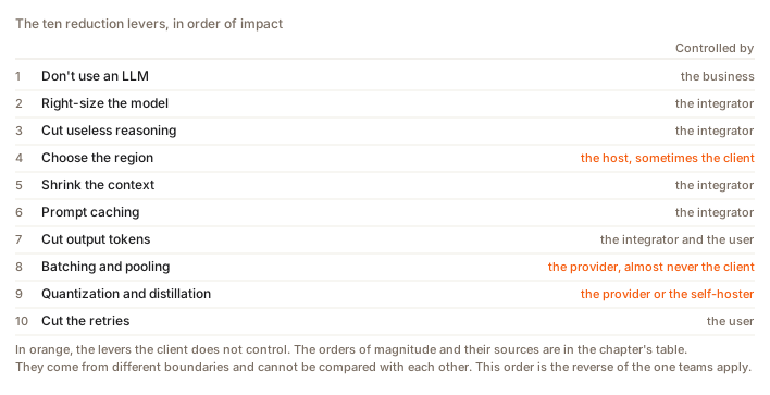
The table, with who controls what
The last column decides what you can act on in a given engagement. The numbers behind each lever come from the chapter on the formula.
| # | Lever | Order of magnitude | Controlled by |
|---|---|---|---|
| 1 | Do not use an LLM | the compute never happens | the business |
| 2 | Do not oversize the model | over 65 between models served by API | the integrator |
| 3 | Switch off unnecessary reasoning | 3 to 30, tails to 700 | the integrator |
| 4 | Choose the region | 14 to 21 on grid intensity, 126 between two sites | the host, sometimes the client |
| 5 | Cut the context | superlinear, low ceiling on agentic use | the integrator |
| 6 | Prompt cache | −80% on price, energy gain not measured | the integrator |
| 7 | Cut output tokens | 48.5% of the carbon of an agentic session | the integrator and the user |
| 8 | Batching and sharing | 17 to 25 between batch 1 and batch 32, around 35 between an unbatched measurement and a production measurement | the provider, almost never the client |
| 9 | Make the model itself lighter | −39%, conditional | the provider or the self-hoster |
| 10 | Cut the retries (prompt engineering) | 32% to 48%, single source | the user |
The cross-cutting lever: measure, then track
None of the ten can be ranked without a meter. The order above comes from measurements published on given models and given hardware; at a client, the orders of magnitude move with the model called, the usage profile and the region. Without measurement you are applying someone else's ranking.
What to record, and what nobody records on their own:
- the three token classes separately, fresh input, cache reads, output, because a single counter overstates by a factor of 3.3 to 3.6 on an agent session;
- the model called, request by request, since lever 2 is the strongest in the table;
- a breakdown by team or by use case, without which no trade-off has an owner;
- the date, so that one quarter compares with the next on the same boundary.
Tracking matters as much as the first measurement. A single reading gives a number, a series gives a trend, and the trend is what tells you whether a lever did anything. It is also the only way to see the rebound effect described below coming.
On tooling, an API provider's usage export gives token volumes and the model called, which is enough to start. For continuous tracking by team, with the three token classes and a dated emission factor, that is what TokenClimate does, which I build.
Lever 1: do not use an LLM
The most frugal compute is the compute that never happens, and a good share of deployed use cases have a deterministic substitute that is cheaper, more reliable and auditable.
How was it done before? A tool may already exist, or a short script, or a dashboard. Then, by increasing cost: character recognition, business rules, vector search without generation, a small specialised model. The frontier model comes last, and only if none of the others is enough.
A number to place the rungs, measured by Luccioni, Jernite and Strubell (Power Hungry Processing, FAccT 2024) on one A100 card of an eight-card node, with no request batching, in kWh per thousand inferences: classifying text 0.002, extractive question answering 0.003, generating text 0.047, generating an image 2.907. Generating rather than classifying uses about twenty times more energy (23.5 as a ratio of means, about 18 as a ratio of medians).
The first rung is a question, not a technique: does the need really call for a feature built with AI, or something else, or nothing at all. The first deliverable of a sufficiency review is the list of use cases that never needed a frontier model.
Lever 2: do not oversize the model
The gap between models served by API exceeds 65 from the most frugal (Llama-3.1-8B) to the greediest (DeepSeek-R1), on long prompts, across the 30 models in Jegham et al., How Hungry is AI? (v6, November 2025). Those values are estimates, not measurements: API latency plus inferred hardware attribution. Quote them with that limit attached.
Providers do it for themselves. At Google, the strategy is to route consumer requests to smaller models as soon as a new generation matches the previous one's performance. For product integrations, it is never the generalist models running but specialised versions.
Three limits to state, two of them awkward. Economic lock-in: investment in data centres sized for large models creates pressure to earn that money back. The training legacy: many small models are distilled from large ones, which reduces their upstream benefit. And a stacking risk: if small models get added to large ones rather than replacing them, the gain evaporates. Ask for proof of replacement.
Lever 3: switch off unnecessary reasoning
Reasoning mode costs 92% more energy on average, and up to 849% more on a code generation task, for a performance gain that varies by task. On tasks where it adds nothing, it is pure overhead.
And even where it does add something, half of it is surplus: a published method brings the token volume from 2,408 down to 1,331 on a maths set, −44.7%, for an accuracy of 92.8% against 93.0%.
This is an API parameter, not a project. Measure at the client before recommending a level: the same task set at the different settings, reading the output token counter. One afternoon, and you have the only number that matters, the one for their tasks.
Lever 4: choose the region
Same energy, same model, same code. Only the electricity mix changes.
Two different quantities circulate under this one lever, and confusing them wrecks the argument.
The intensity ratio between grids is 14 at Ember (production, LCA, 2025) and 21 at Electricity Maps (traced consumption, LCA, 2025) between France and Poland. That is a factor per kilowatt-hour, and it survives the choice of database, which is rare.
The annual inventory ratio between two sites is 126: Meta publishes its location-based scope 2 emissions per data centre for 2024, and the gap between Luleå in Sweden (5,298 tCO2e) and Altoona in Iowa (666,434 tCO2e) reaches that factor, at the same operator. That number aggregates grid intensity and the volume of electricity consumed at each site: per kWh, the gap falls to about 37, by our calculation. It illustrates the lever, it does not measure it.
Three limits, rarely stated.
This lever has a scale ceiling. Lin et al. (2023) note that hyperscale data centres exceed 15% of the load on some regional grids; at that size, moving the load towards decarbonised electricity disturbs the very grid you are trying to spare. The lever works for one player alone, not for everyone at once.
On the total footprint, this lever returns less than the ratio of the grids: from the AWS region assumed for Anthropic to the French grid, the composite only falls by a factor of 3.9 by our calculation, not 14 or 20, because the hardware's carbon does not change. The cleaner the starting grid, the more that floor weighs.
And on a proprietary API, you do not choose the region. The lever is real for self-hosting or a cloud with region selection, unavailable for most usage.
Lever 5: cut the context
The cost of context is superlinear, and providers bill it with a 2× multiplier on input beyond their threshold. Routing each question to a targeted search rather than to the full context cuts input token volume by 61.6% on Gemini 1.5 Pro, against the full long context and at a cost of 3.3 quality points, with a hybrid method (Self-Route) that falls back to the long context when retrieval is not enough, in Li et al. (Google DeepMind, EMNLP 2024), across nine datasets.
The gain is in tokens, not joules, and the retrieval pipeline is not free. And on agentic use the ceiling is low: fresh input and cache writes are 28.8% of the footprint, so a perfect compressor applied to new tokens only, without touching the history already in cache, does not get below 71% of the total.
Lever 6: prompt cache
A gain with no quality loss at all, which makes it unusual: the result is identical, it is the compute that disappears. Announcements go as far as 90% off the cost of the tokens concerned, and the measurement by Lumer et al. (Don't Break the Cache, arXiv:2601.06007, January 2026) across more than 500 agent sessions from the DeepResearch Bench gives −79.6% on the full GPT-5.2 bill.
The boundary trap is here. The cache removes prefill, that is, the cheapest part per token, about 35 times cheaper than an output token at batch size one. A 90% discount on the price of input tokens is not 90% of energy saved.
Only one measurement compares the energy of a cache hit with that of a miss, Irminsul, on a 4,096 token prefix, far from an agent's contexts. Defensible position: the cache reduces the compute actually performed without degrading the output, its energy magnitude at agent scale is not measured, and it is lower than the commercial discount.
The cache is a prefix: anything that changes the start of the context mid-session invalidates it for everything after, so add nothing along the way. The duration counter starts at the beginning of the request, not at the end of the answer. And the pricing models differ, one charging for writes, another for hourly storage.
Speculative decoding, same family, same trap
A small "draft" model proposes several tokens ahead, the large model checks them in a single pass and keeps the longest prefix consistent with what it would have produced itself.
Same property as the cache: at zero temperature, when the model always takes the most likely token, the output is strictly identical. This is not an approximation, it is a rearrangement of the compute. Published speed-ups run from 2 to 3.6 times, all measured in latency: 2 to 3 times in Leviathan, Kalman and Matias (arXiv:2211.17192, ICML 2023) on T5-XXL at batch size one, up to 3.6 times for Medusa (arXiv:2401.10774).
The trap is nastier than the cache one, because it can reverse the gain. The only two published energy measurements give −12% to −27% with a well-matched draft (Nik, Riegler and Halvorsen, SimulaMet, arXiv:2502.11723, peer-reviewed version Scientific Reports 2026; Qwen2.5-7B on an A100, n-gram draft, greedy decoding), and 30% more consumption despite a 1.19 times speed-up when the draft is badly matched (Dutta et al., arXiv:2602.09113, Findings of EACL 2026; Vicuna-7B on an A5000, CodeCarbon measurement). Both run at batch size one, the most favourable regime.
Speed and energy do not necessarily move together, then. Like batching, this lever belongs to the provider.
Lever 7: cut output tokens
An output token uses about 35 times the energy of an input token, measured at batch size one. On an agentic session, output is 0.73% of the volume and 48.5% of the carbon.
Three ways to act: constrain the answer length and switch off reasoning, but also pick a model that answers briefly. That last point is poorly known: on the same task, models produce answers of different lengths, and that verbosity appears in no comparison grid anywhere.
One trap worth knowing. Optimising joules per token encourages generating more, since the fixed costs get amortised: Vellaisamy et al. (Carnegie Mellon) measure on Qwen3-8B and MATH-500, on an H200, 7.46 J per token at 10 output tokens against 0.72 J at 512, while the energy of the request is multiplied by 5. Optimise joules per task solved.
Lever 8: batching and sharing
Decoding is memory-bound, so handling several requests in the same pass amortises reading the weights. Two distinct quantities, to be given separately.
The gain runs from 17 to 25 between batch 1 and batch 32, depending on the attention architecture (Ma et al., The Illusion of Power Capping in LLM Decode, May 2026; one H200, models of around 4 billion parameters, decode phase isolated).
The total observable gap between an unbatched measurement and a production measurement reaches around 35 on models of the same class. That one compares two complete protocols, not two batch sizes: 1.72 Wh per request on Llama-3-70B at AI Energy Score against 0.0486 Wh on Llama 3.3 70B at ML.Energy v3.0. The weights are not exactly the same, the order of magnitude holds.
Hence a counter-intuitive conclusion: self-hosting a model at low volume is worse energetically than calling a shared API. The numbers: when generating, an H200 draws only 137 to 300 W out of 700, from batch 1 to batch 32, energy per token at batch 1 is 17 to 25 times that of batch 32, and on BLOOM, measured over 18 days on 16 A100s with no batching, roughly 75% of the energy goes simply to keeping the model in memory (Luccioni, Viguier and Ligozat, JMLR 2023).
Two caveats, or you are selling cloud. First, separate this physical argument from the hyperscalers' marketing argument, which compares their fleet with a deliberately inefficient installation. And at high volume with steady load, self-hosting becomes defensible again, with levers the API forbids. The threshold can be calculated.
Lever 9: make the model itself lighter
Reducing numerical precision to 8 bits gains 39% on average according to the estimate by PEReN for Arcep, the French telecoms and digital regulator (May 2026, 22 open models on the Jean Zay supercomputer, GPU only). And distillation gains 83% to 90% of inference energy for 13 to 15 ROUGE-L points lost, on CodeT5+ and an RTX 4090 (arXiv:2608.17515).
The result that stops you recommending it blind: at small batch, between 8 and 16 requests, reduced precision consumes more than standard precision in 7 measured cases out of 7, with a median of 30% more (ML.Energy v3.0, observation 7, H100 and B200). The gain only shows up at large batch. Low precision only pays in compute-bound regimes; in a memory-bound regime it pays nothing.
On quality, do not repeat the "negligible degradation" of the method papers. The most honest source is Meta's, which writes that standard benchmarks do not properly reflect the effects of quantisation, and that without guardrails the model occasionally produces corrupted answers while the scores stay good.
Lever 10: cut the retries
A failed answer is energy spent for nothing, plus a second request. In a conversation, the retry costs more than the initial request, since the whole history goes back up the wire.
Prompt engineering is energy saved too, in the literal sense: a prompt that gets the right result first time removes entire requests. A piece of green prompting work, Podder, Date and Murthy (Environmental Science and Ecotechnology, March 2026), measures 32% to 48% less inference energy when its prompt best practices are applied, across several models and scenarios. The Arcep report of May 2026 writes "up to 50%" instead, citing UNESCO (2025). A single study behind the number.
The moves that work. Frame it once rather than ten round trips: a longer but precise prompt costs less than a short prompt that forces iteration, since input uses 35 times less energy than output at batch size one, and costs about 5 times less. Write every prompt as if you had one shot, and send text rather than a scanned document. Last point, do not fill the window to the brim: quality degrades well before the technical limit, so retries go up. MISSING DATA on the threshold: no published measurement links fill rate to error rate. It would take running the same evaluation at several fill rates, with the model and task held constant.
The limit to state, or this lever becomes manipulation: its real value is educational, it makes the subject tangible for a user who chooses neither their model nor their region. Its risk is shifting responsibility onto the end user while the factor-of-10 decisions get taken elsewhere. Putting it tenth is not an accident, and you should say so out loud when you present it.
Question
A client wants to cut the footprint of their internal assistant and gives you one day. Where do you start?
Choisissez une réponse pour voir l'explication.
The fake lever you will be offered
Temperature controls how the next token is drawn (chapter 1): low, the model almost always takes the most likely token; high, its answers vary more. A more predictable model feels like it is doing less work, hence the idea of lowering the temperature to consume less. It does not work.
Technically, temperature is a division of the scores, applied after all the compute, on a vector the size of the vocabulary. It adds no layer, no pass, no weight read. Its cost is negligible next to the rest.
Measurement confirms it: Nik, Riegler and Halvorsen (SimulaMet, arXiv:2502.11723, peer-reviewed version Scientific Reports 2026) sweep temperature from 0.1 to 1.2 on Qwen2.5-7B, two A100-PCIE-40GB, batch size one, and find a spread of −0.2% to +2.6% against greedy decoding depending on the task. Noise. On the same rows, switching to the DoLa decoding strategy costs 51.5% more.
Two indirect channels do exist. A high temperature can make the model write for longer, and the cost is then in the token count, not in the setting. It also degrades the acceptance rate of speculative decoding: EAGLE-2 (arXiv:2406.16858) measures a speed-up loss of 5.4% to 21.6% going from zero temperature to 1, on the badly matched pairs only. Nobody has measured the chain from there to energy.
Nobody has measured average output length as a function of temperature with the model and prompt held fixed. MISSING DATA. The experiment takes two days for anyone with a GPU: output length and how often the model stops on its own, at several temperatures, on a fixed set of prompts.
What this list does not settle
Efficiency per process tells you nothing about the consumption of the system. Google divided the energy of its median request by 33 between May 2024 and May 2025. Over 2025, its data centres' electricity consumption rose 38% and its total emissions, under its "ambition-based" scope, 18%. The ten levers above are real and quantified, and all of them have been pulled at scale by the players who master them best.
Left to voluntary action, one party's frugality frees up capacity for another. Only a constraint on the total, a cap or a binding budget, beats a rebound effect.
Individual levers exist and are quantified, but on their own they do not bring the total down.
To apply this ranking to real usage, the calculator quantifies a mix of models and the methodology publishes the parameters used.
FAQ
What is the most effective lever for reducing the footprint of AI?
Not using a language model when a deterministic substitute is enough, since the compute then never happens. Model choice comes next, with a gap of more than 65 between the most frugal and the greediest model, estimated by Jegham et al. across 30 models served by API, on long prompts. Prompt optimisation comes tenth, with a gain that rests on a single study.
Does optimising your prompts really reduce the carbon footprint?
Yes, on exchanges that forced retries, but the evidence is thin. Podder, Date and Murthy (2026) measure 32% to 48% less inference energy when their prompt best practices are applied, mostly because they avoid starting over. The Arcep report of May 2026 writes "up to 50%", citing UNESCO. One published measurement, and a gain limited to tasks where people were starting over. Its real value is educational: it makes the subject tangible for a user who controls nothing else.
Should you self-host a model to reduce its footprint?
Not at low volume, where it is worse energetically than a shared API. When generating, an H200 draws only 137 to 300 W out of a 700 budget, even batching up to 32 requests, and one request at a time more than 88% of its tensor cores sit idle, while roughly 75% of the energy goes to keeping the model loaded. At high volume with steady load, the trade-off flips.
Does switching off reasoning mode degrade quality?
On tasks that do not warrant it, no: the PEReN study for Arcep estimates an average overhead of 92% energy, with a wide interval, for a performance gain that varies by task. And even where it does help, a published method removes 44.7% of the reasoning tokens for an accuracy loss of 0.2 points. The setting should rest on an evaluation, not on intuition.
Are efficiency gains enough to bring down the total footprint of AI?
No, and the best counter-example comes from a provider. Google divided the energy of its median request by 33 between May 2024 and May 2025, while, over 2025, the electricity consumption of its data centres rose 38% and its total emissions 18% under the "ambition-based" scope of its 2026 Environmental Report. Only a constraint on total volume, as a cap or a budget, offsets a rebound effect.